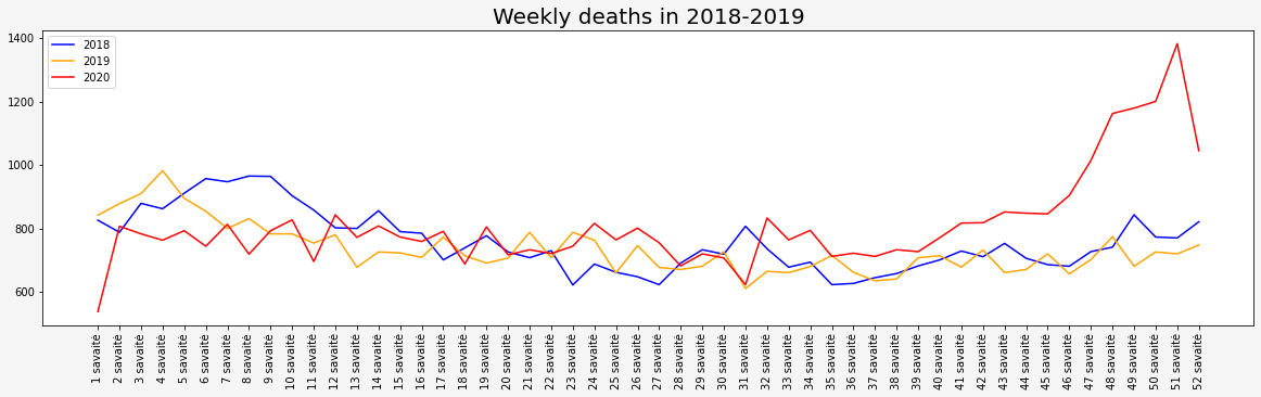
Recently I posted a chart of weekly deaths in 2019 and 2020. There were some doubts that it is not correct to compare 2020 versus 2019. The proposal was to take an average of some period of years and compare it to 2020. It is a great suggestion! It was my intention to compare it with the previous year.
However, I kept thinking if there is a significant difference between 2018 and 2019. In that case, my previous post is nonsense.
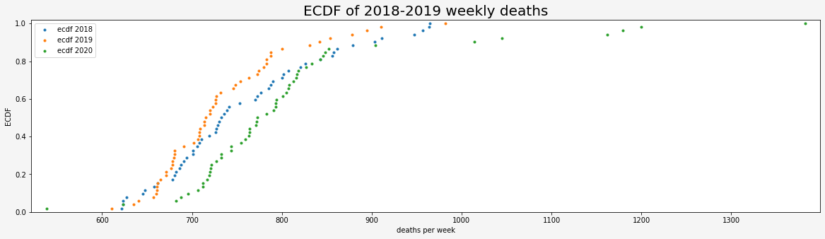
A few weeks ago, I found “hacker statistics” as an ingenious way to prove a point. I think I heard this term for the first time, but honestly, it is just a statistical analysis that relies mostly on simulation or resampling for inference. So I tested a hypothesis (H0) that the means of weekly deaths in 2018 and 2019 are equal in both ways (with “hacker statistics” and Two-Sample t-Test). Firstly, I visualize my data. I plotted weekly deaths for 2018, 2019, and 2020. Then I drew ECDFs for each year.
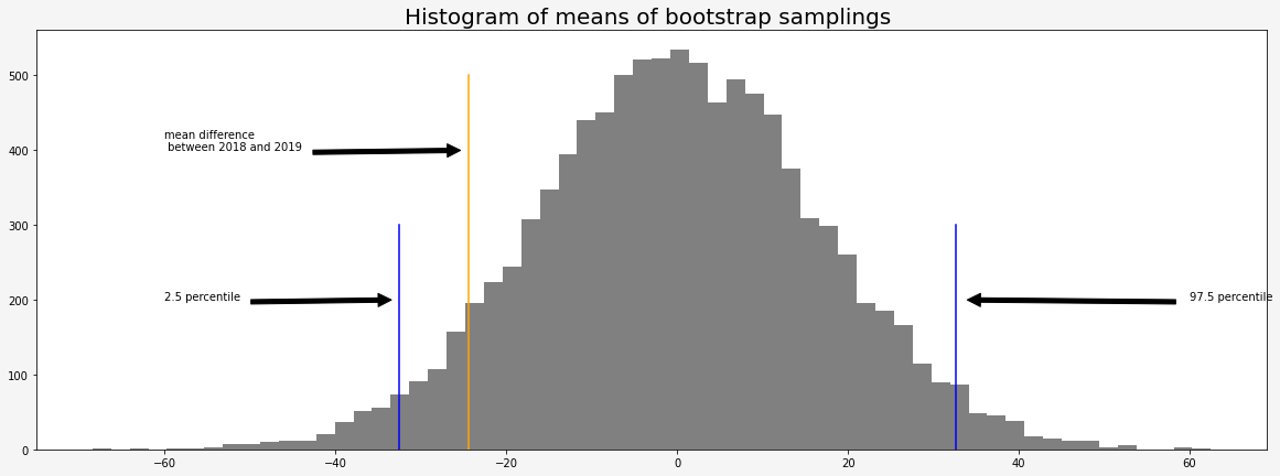
The absolute difference between the means of 2018 and 2019 weekly deaths is -24.38 deaths per week. To perform my hypothesis test in the “hacker statistics” approach I shifted two data sets to have the same mean and then used bootstrap sampling to compute the difference of means.
Wikipedia: “Bootstrapping is any test or metric that uses random sampling with replacement, and falls under the broader class of resampling methods. Bootstrapping assigns measures of accuracy (bias, variance, confidence intervals, prediction error, etc.) to sample estimates. This technique allows estimation of the sampling distribution of almost any statistic using random sampling methods.”
I generated 10 000 means of weekly deaths in 2018 and 10 000 means of weekly deaths in 2019. With these data sets, I got 10 000 differences of means. The last step is to calculate p-value. And the result is p = 0.06889.
It was a fun exercise to create the simulation. But as a mathematician, I would like to show this with a proven statistical method. With Python, it is easy to perform a t-test within a few lines.
The two-sample t-test for weekly deaths is defined as:
H0: μ1=μ2
H1: μ1≠μ2,
where μ1 is average weekly deaths for 2018 and μ2 is average weekly deaths for 2019. The result is p = 0.1486. A p-value higher than 0.05 (> 0.05) indicates strong evidence for the null hypothesis.
I performed the test for weekly deaths in 2019 and weekly deaths in 2020 (with Covid19 deaths and without Covid19 deaths). For both data sets of 2020 H0 hypothesis was rejected (i. e. death average was significantly different).
So, the other question - what is the Covid19 impact on other deaths. Pearson correlation for 2020 between Covid19 cases and other deaths is 0.72. It shows a strong linear relationship between those two. The regression line is with a slope of 0.013 and an intercept of 745.803.
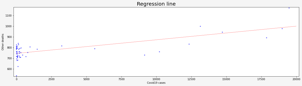
This means that for every 100 Covid19 cases there are 1,3 additional deaths from other reasons than Covid19. So if on some week we had 17 000 cases we might expect 221 deaths from other illnesses (after some time) on top of the expected average (700) without the Covid situation. Additionally, we have 2% Covid19 mortality (340). So in total, we get more than 1200 deaths per week…
So please, stay at home. Even if you think that Covid19 is the same as Flu - you might save someone’s life.